Evaluating Service Compliance Using Error Rate
Calculate and Aggregate Error Rate
To illustrate, consider the following example:
Example:** Up to the current time (T = 15m), 21 events corresponding to data points have been collected, where X data points are bad events and Y data points are good events. These data points are arranged as follows on a time-series:
 *+**+*+ ****+** +*+*++* ****+
|---------------------------->
0m                          15m

(*) represents a good event
(+) represents a bad event.
When evaluating the Error Rate (ER), it’s important to assess it over time windows. For instance, in this case, each evaluation considers a time window of 5 minutes (time_window=5m). The values are still arranged as initially shown but grouped into time segments:
 *+**+*+ ****+** +*+*++* ****+
|-------|-------|-------|---->
0m     5m      10m     15m  ...
Overlap can occur in data points when assessing with smaller time windows using a rolling-window mechanism.
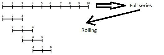
To address this issue, simply ensure that the interval between evaluations is >= time_window. However, this will increase the detection time because interval will equivalent to time to return evaluation result. Thus, a higher interval will result in longer detection times.
 *+**+*+ ****+** +*+*++* ****+
|-------|-------|-------|---->
0m     5m      10m     15m  ...
       (1)     (2)     (3)
        ^       ^       ^
        |       |       |
---(G1)-+--(G2)-+--(G3)--
                |
                v
      ______________________
     |                      |
     | Error rate aggregate |
     |______________________|

Legend:
  tw: time window (= 5m)
  (1) (2) (3): Times of ER collection (n)
  (G1) (G2) (G3): Groups of data points considered in each corresponding evaluation (chunks)
The groups of data points allocated per time window are represented as shown above, dividing the 15m period into 3 evaluation stages corresponding to groups G1, G2, G3. From there, the aggregated Error Rate from each time window is calculated as follows:
Error rate aggregate phase:

----------------------------------------------------------------------------------------
|   n   |  chunks  |   time range   |  total event  |   bad event    |    error rate    |
---------------------------------------------------------------------------------------
|  (1)  |    C1    |     0m -> 5m   |      7        |        3       |       0.42       |
|  (2)  |    C2    |     5m -> 10m  |      7        |        1       |       0.14       |
|  (3)  |    C1    |     10m -> 15m |      7        |        4       |       0.57       |
========================================================================================
The example simulates events that are evenly distributed across time segments, but reality will be different. However, the way to aggregate ER is completely similar.
Therefore, the error rate index needs to be cross-referenced with the Error Budget to compute the amount of Error Budget Remaining for the service. For instance, if at an evaluation stage (t), ER = 0.42 is obtained, how much EB does this ER “burn”?
Evaluating service compliance
The EBR value at the start of each cycle is initialized with 100% EB. This means, if you have EB = 33.6h per month, equivalent to 6.72h EB per cycle (week), each cycle starts with 6.72h EB and resets at the end of each cycle. Whenever a bad event occurs, the amount of EBR decreases until it reaches 0 (exhausted). If EBR is exhausted earlier than expected, the service violates compliance.
-> So, how is the amount of EB exhausted based on the calculated ER?
For clarity, using the example above, in the initial evaluation stage, ER = 0.42 (42% of events are bad) within 5 minutes. This allows us to calculate the Error Budget consumed and the Error Budget Remaining:
At time t:

EB(consumed)[t] = ER[t] * time_window = 0.42 * 5 = 2.1 (minutes)
EBR[t] = EBR[t] - ER[t] = 6.72h - 2.1m = 6.685 (hours)
-> Therefore, a 42% Error Rate will consume 2.1 minutes of Error Budget.
Applying this calculation method allows us to deduce EB(consumed) and EBR at subsequent evaluation stages:
Error rate aggregate phase:

-------------------------------------------------------------------------------------------------------------------------------------------------------
|   n   |  chunks  |   time range   |  total event   |   bad event    |    error rate    |   EB consumed (by minutes)   |      EBR (by hours)         |
-------------------------------------------------------------------------------------------------------------------------------------------------------
|  (1)  |    C1    |    0m -> 5m    |       7        |        3       |       0.42       |           2.1                |             6.685           |
|  (2)  |    C2    |    5m -> 10m   |       7        |        1       |       0.14       |           0.7                |             6.673           |
|  (3)  |    C3    |    10m -> 15m  |       7        |        4       |       0.57       |           2.85               |             6.6255          |
=======================================================================================================================================================